Project 1

03/01/2021

A description of the housing data you scraped from zillow

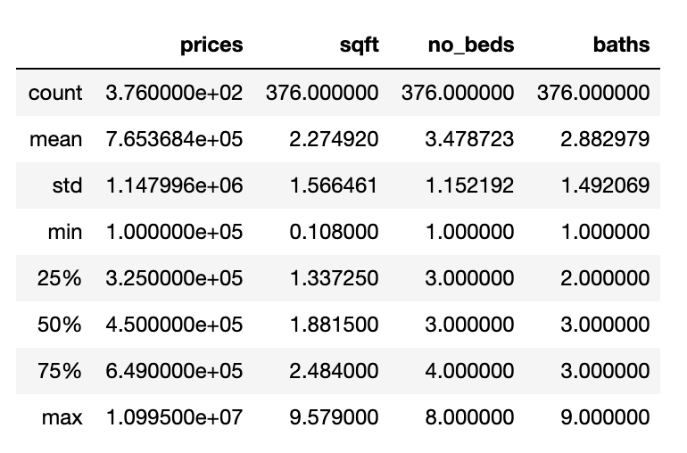
I initially had 400 data points, but had to remove some due to incomplete or unusable date. Ultimately, I ended up with 376 data points corresponding to different homes in Austin, Texas. Each data point had information about its price, address, number of beds, number of baths, and its squarefootage. These data points were loaded into a csv file and then used to create a pandas dataframe. Here are some descriptive statistics about the collected data:

A description of your model architecture

Before building the model, I preprocessed the data into a form usable for the model. This included dropping a couple of bad data points as well as dividing all the values for squarefoot by 1000. Next, I created numpy arrays named x1, x2, and x3 that corresponded to each of the 3 features number of beds, squarefootage, and number of baths respectively. I next stacked them together into a variable called xs and made a variable called ys that included all the corresponding prices for the houses. I imported Tesorflow in order to help build the model. Next, I initialized the keras Sequential model with an input shape of 3. I then compiled the model with a stochastic gradient descent optimizer and mean squared error as the loss function. Finally, I fit the model based on the values in my xs and ys variables with 500 epochs.

At this point, my model had been created, and it was time to start pretictions. I used the same data points that were utilized to train the model to test it, and added the predicitons in another column to the original dataframe. Next, I created one more column called difference that held the value of predicted price minus the true price.

An analysis of your model output

The model that I built was not super accurate for the most part, which I think is somewhat expected with only 3 features being used in predictions. The MSE values that I calculated tended to be pretty high. The 10 biggest over-predictions had an MSE of 535562223415.2863, and the 10 biggest under-predictions had a value of 23479729427135.414. Even the 10 most accurate results still had a pretty large MSE of 69908328585.21533.

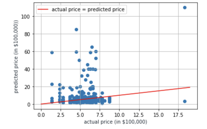
As seen by the graph below, a lot of the data points lie far away from the red line, which designates the points where the actual price is equal to the predicted price. Any value that lies above the line represents a home in which the predicted price is greater than the actual price, which corresponds to a good deal. Similarly, any value that lies below the line represents a home in which the predicted price is lower than the actual price, which corresponds to a bad deal. The closer the data point is to the line, the more accurate the modek was in predicting its price!

An analysis of the output that assesses and ranks all homes from best to worst deal

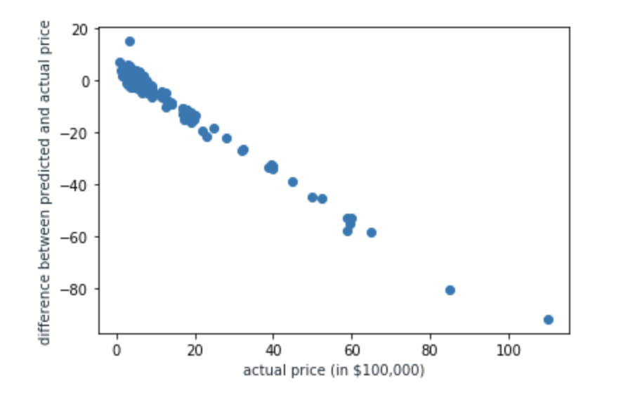
The graph below shows each home along with the difference between the predicted value for its price and the actual value for its price. The greater the difference, the better the deal, and the more negative the difference, the worse the deal. Essenitally this means, values that are toward the top of the graph are better deals than those at the bottom.

As is clear with this graph, the model made quite a few underpredictions in which it predicted the price to be much smaller than its actual price. This may have to do with location because smaller homes could still be fairly expensive in certain neighborhoods, and the model wasn’t able to take this into account. There are definitely many ways I could build upon this model to improve its accuracy, but I think it was pretty successful given the amount of data that was utilized!